How to Add Line Breaks in latex Equations

LaTeX is a widely used typesetting system, especially for documents that require precise formatting of mathematical equations. Its ability to handle complex mathematical notation with accuracy makes it the go-to tool for academics, scientists, and engineers. However, when equations become too long, they can compromise both readability and structure, leading to confusion.

Properly formatting equations by introducing linebreaks helps maintain clarity without altering the mathematical meaning.

In this tutorial, I’ll explain various methods to break long equations into multiple lines in LaTeX. You’ll learn how to control equation alignment, manage numbering, and fine-tune spacing to make complex equations more readable and well-structured.

Using \ for Single Equation Linebreaks

In LaTeX, when equations are too long to fit on a single line, you can introduce linebreaks to improve readability using the \\ command.

This is the most straightforward way to split equations into multiple lines. However, the way LaTeX handles these breaks varies depending on the environment you’re using, and it’s important to understand the impact on alignment and numbering.

Using \\ in the equation environment:

The equation environment is ideal for single equations that need to be centered on the page. When you use \\ within this environment, LaTeX breaks the equation into multiple lines but centers each new line by default. Here’s an example:

\begin{equation}
a^2 + b^2 = c^2 \\
+ d^2
\end{equation}

This will be rendered as:

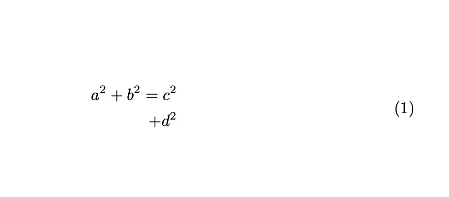
In this case, the first part of the equation will appear on the first line, and the second part (+ d^2) will appear directly below it, but centered. While this works for short breaks, it can become visually unbalanced when splitting larger expressions, as LaTeX doesn’t provide control over how lines are aligned within the equation environment.

Impact on equation numbering:

Understanding how LaTeX handles equation numbering is essential when breaking long equations.

• In the equation environment, even if an equation spans multiple lines, LaTeX assigns a single number to the entire equation. This is often preferable when the equation is conceptually a single entity.
• In contrast, the align environment(Explained in next section) treats each line as a separate equation by default, giving each line its own number.
• You can use \nonumber to skip numbering for specific lines if you want only certain lines to be numbered. In this form, no line numbers will appear, which is useful when equation numbering isn’t required or might clutter the layout.

Understanding the differences between the equation and align environments helps you manage how your equations are broken, aligned, and numbered, ensuring clarity and proper formatting in your LaTeX documents.

Using align and multline for Handling Multi-line Equations

When working with complex or long equations in LaTeX, the amsmath package provides powerful environments to manage multiple lines and improve readability.

Two of the most useful options are the align and multline environments, each designed for different needs.

Using the align Environment:

The align environment is ideal for equations that require precise alignment of terms, such as systems of equations or long expressions with multiple components. By using the & symbol, you can easily align terms at specific points, like equal signs or operators, making the structure clear and easy to follow. Here’s an example:

\usepackage{amsmath}

\begin{align}
x_1 + y_1 &= z_1 \\
x_2 + y_2 &= z_2
\end{align}

This will be rendered as:

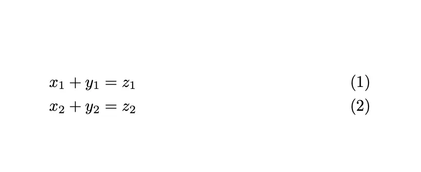
In this case, each equation is aligned at the = symbol. You can suppress numbering for certain lines using \nonumber or remove all numbering by switching to the align* environment.

This makes align versatile for handling both single and multi-line equations that benefit from term alignment.

Using the multline Enviornment:

The multline environment is best suited for breaking long equations that do not require alignment, such as when terms on either side of the equation are unevenly distributed.

It centers each line naturally and wraps the equation as needed. For example:

\begin{multline}
a + b + c + d + e = \\
x + y + z
\end{multline}

This will be rendered as:

Use multline when the structure of the equation doesn’t need to align at specific points but still requires multiple lines for better presentation.

Both align and the multiline environments ensure your equations are readable, whether you need precise alignment (align) or natural line breaks (multline).

Using the split Environment for Sub-equations

The split environment allows you to break an equation into sub-parts, providing clarity for complex expressions while maintaining a single equation number.

This environment is especially useful within the equation environment, as it allows for organized presentation without compromising the overall structure.

When using the split environment,

• Enclose it within the equation environment to ensure the entire expression retains a single centered equation number.
• Each line of the split can contain parts of the equation, enabling you to show logical progression or steps without creating multiple numbered equations.

Here’s an example:

\begin{equation}
\begin{split}
    E &= mc^2 \\
    &= m \cdot (3 \times 10^8)^2 \\
    &= 9 \times 10^{16} \cdot m
\end{split}
\end{equation}

This will be rendered as:

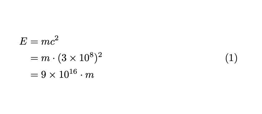
In this example, the equation (E = mc^2) is broken into parts that explain each step. The entire expression maintains a single equation number centered beneath the split lines, ensuring clarity and coherence.

Using the split environment allows for better readability, especially in lengthy derivations or when working with intricate expressions. This way, readers can easily follow the logic without distraction from multiple equation numbers.

Fine-Tuning Linebreaks with the array Environment

The array environment provides fine control over the layout and alignment of elements in equations, allowing you to customize column arrangements and manage line breaks effectively.

This is particularly useful when you want to present multi-part equations or systems of equations with specific alignment requirements.

To create an array, define the structure with alignment characters, such as c for center, l for left, and r for right.

For example, if you want to arrange a system of equations with specific alignment, you can set it up like this:

\[
\begin{array}{rl}
x + y &= 5 \\
2x - y &= 1 \\
3x + 4y &= 9
\end{array}
\]

This will be rendered as:

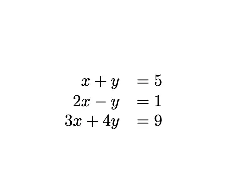
In this example,

• The array environment is configured with rl, indicating that the first column is right-aligned and the second column is left-aligned.
• Each line break occurs naturally, allowing for clear separation of equations while maintaining a neat alignment.

You can also use the array environment to customize line breaks within more complex expressions.

For instance, if you want to display a single equation broken into parts with controlled alignment, you might structure it like this:

\[
\begin{array}{rcl}
a + b + c &=& d + e + f \\
& & g + h
\end{array}
\]

This will be rendered as:

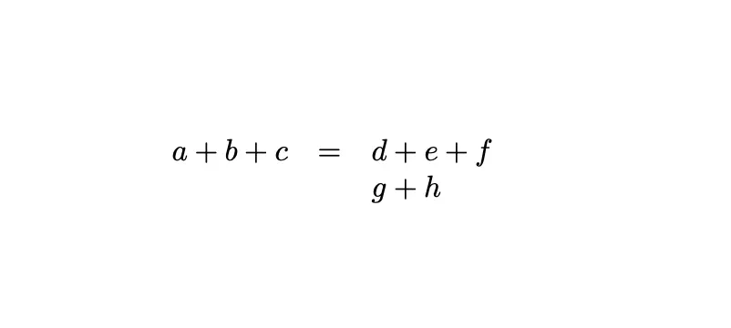
Here:

• The first column is right-aligned, which helps emphasize the equation’s progression, while the second column aligns the equal signs.
• The third column demonstrates how to break the equation into additional components, allowing for clarity and a structured presentation.

By leveraging the array environment, you can fine-tune the appearance of your equations, ensuring that they are not only mathematically accurate but also visually appealing and easy to follow. This method enhances readability, particularly in complex formulations or when conveying multiple relationships within a single framework.

Managing Long Equations with cases

The cases environment is an effective tool for managing long equations, especially when dealing with piecewise functions.

It allows you to clearly define different conditions under which specific equations apply, making it easier for readers to understand the function’s behavior across various scenarios.

To use the cases environment, you can structure your equations by providing conditions alongside their corresponding expressions. This layout not only organizes your equations neatly but also enhances readability by clearly delineating different cases.

You can create this piecewise function using the cases environment like this:

\[
f(x) =
\begin{cases}
x^2 & \text{if } x < 0 \\
2x + 1 & \text{if } 0 \leq x < 3 \\
9 & \text{if } x \geq 3
\end{cases}
\]

In this example,

• Each line corresponds to a different case of the function, with the condition clearly stated beside the respective expression.
• The use of the & character aligns the expressions and conditions neatly, allowing for a clean presentation.

When equations become lengthy or complex, the cases environment provides a structured format that improves comprehension.

This is especially helpful in mathematics and engineering, where functions often have multiple definitions based on varying inputs.

By using the cases environment, you can enhance both the clarity and the accessibility of your equations, making it easier for readers to grasp the underlying concepts.

Handling Equation Spacing with !, \quad, and \hspace

Proper spacing in equations enhances readability and clarifies relationships between elements. LaTeX provides several commands to fine-tune spacing, including \!, \quad, and \hspace, each serving distinct purposes.

The command \! reduces the space between elements, which is particularly useful when you need to bring terms closer together. For example, if you have an equation where the spacing seems too wide, you can use \! to tighten it:

\[
A = B \! + C
\]

In this example, the \! command pulls C closer to the B + term, which may be preferable for stylistic reasons or to enhance clarity in specific contexts.

Conversely, \quad adds a significant amount of space (approximately the width of the letter “M”). This command is useful for separating terms or groups of terms for better visibility. For instance, you might want to clearly distinguish between different parts of an equation:

\[
A = B \quad \text{(where B is a constant)} \quad C = D + E
\]

The \quad command adds ample space between the equations, making it clear that they are distinct statements.

This will be rendered as:

The \hspace command allows for even more precise control over spacing by specifying a custom distance. This command can be used when you need a specific amount of space, whether it’s to conform to style guidelines or to enhance readability. For example:

\[
A = B + \hspace{10pt} C
\]

This will be rendered as:

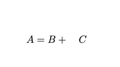
In this case, \hspace{10pt} adds exactly 10 points of space between B and C, which can help avoid crowding in complex equations.

By using these spacing commands effectively, you can significantly improve the clarity and appearance of your equations, making them easier to read and understand. Properly adjusted spacing not only enhances the overall aesthetic but also aids in conveying mathematical relationships more clearly.

Using Inline Math Mode for Wrapping Equations

Inline math mode in LaTeX allows you to seamlessly incorporate mathematical expressions within the flow of text. However, handling line breaks in this mode can be challenging, as LaTeX does not allow for natural line breaks within inline math without disrupting the surrounding text.

When you use inline math mode with single dollar signs ($...$), long equations may extend beyond the line width, leading to issues with readability. For example:

The equation $y = mx + b + \sqrt{a^2 + b^2 + c^2 + d^2 + e^2 + f^2}$ is crucial.

In this case, if the equation is too long, it will not break naturally, and part of it might overflow the text margin.

One common workaround for this limitation is to use the \linebreak or \newline commands, but these do not function properly within inline math mode. Instead, if you find yourself needing to break a long equation, it’s better to switch to display math mode using double dollar signs ($$...$$) or the \[...\] syntax. This provides more room for the equation and allows for natural line breaks:

The equation
\[
y = mx + b + \sqrt{a^2 + b^2 + c^2 + d^2 + e^2 + f^2}
\]
is crucial.

This will be rendered as:

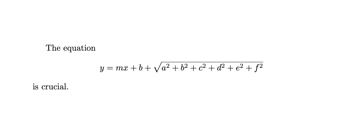
If you still prefer inline math but anticipate a long expression, consider abbreviating parts of the equation or using notation that simplifies the presentation without sacrificing clarity.

Ultimately, while inline math mode offers convenience for brief expressions, be mindful of its limitations with longer equations. Transitioning to display mode not only improves readability but also maintains the aesthetic quality of your document. By strategically choosing when to use each mode, you can enhance the overall presentation of your mathematical content.

Conclusion

Different methods for adding line breaks to equations in LaTeX include:

• multline: Best for long equations without alignment. Automatically centers lines.
• split: Useful for sub-part alignment within a single equation number.
• cases: Ideal for piecewise functions, presenting conditions and expressions clearly.
• Spacing Commands: Use \!, \quad, and \hspace to adjust distances for clarity.
• Inline vs. Display Math: Use inline for brief expressions, and switch to display mode for longer equations to prevent overflow.

Choose the method based on the equation’s complexity and presentation needs to maintain clarity and readability.

See Also

• Wrap Text in LaTeX Tables